
ex2_1プログラム
簡易的なフィルタによるランダム雑音の除去
% Attenuation signal
alpha=300;????? % alpha:attenuation constant
fc=200;??? % fc:carrier frequency
% obserbvation time: 0 to 20ms
% Number of samples: 200samples
t=linspace(0, 0.02, 100);
x=exp(-alpha*t).*sin(2*pi*fc*t);
figure(1);
plot(t,x);grid on
xlabel('Time [sec]');
ylabel('Attenuation signal x(t)');
% Different frequency : 220Hz
% Different alpha: 330
fc=220;
alpha=330;
t1=linspace(0, 0.02, 100);
x=exp(-alpha*t1).*sin(2*pi*fc*t1);
figure(2);
plot(t1,x);grid on
xlabel('Time [sec]');
ylabel('Attenuation signal x(t)');
ex2_2プログラム
2次元フィルタリングによる雑音抑圧
% Test Pattern? (Grating)
clear;
W=512; %横幅
H=512; %縦幅
I1=zeros(H,W);
I_center=128;
I_mod=128;
f_start=0; % 最低空間周波数
f_stop=50; % 最高空間周波数 cycle/W
f_w=f_stop-f_start;
for x=1:W;
for y=1:H;
r=sqrt(((x-1)/W)^2+((y-1)/H)^2);
I1(y,x)=I_center+I_mod*cos((2*pi*f_start+pi*f_w*r^2))+randn*100;
end
end
figure(1)
imagesc(I1,[0,256]);colormap(gray)
for loop =1:3;
if loop==1;
% Filter(A)
filter=(1/9)*[1 1 1; 1 1 1; 1 1 1];
else
if loop==2;
% Filter(B)
filter=(1/10)*[1 1 1; 1 2 1; 1 1 1];
else
% Filter(C)
filter=(1/16)*[1 2 1; 2 4 2; 1 2 1];
end
end
% Filtering
I2=zeros(H,W);
for x=2:W-1;
for y=2:H-1;
M=I1(x-1: x+1, y-1:y+1);
F=M.*filter;
I2(y,x)=sum(F(:));
end
end
figure
subplot(1,1,1); imagesc(I2,[0 256]); colormap(gray)
end
ex2_3プログラム
閾値処理による雑音除去
% Bilevel signal (NRZ signal)
clear;
R=rand(1,10);
NRZ=2*round(R)-1;
tn=[0:99];
for n=1:100;
i=fix((n-1)/10)+1;
s(n)=NRZ(i)+0.1*randn;
end;
figure(1)
subplot(2,1,1)
plot(tn,s);grid on
axis([0 100 -1.1 1.1]);
xlabel('Time t');
ylabel('Received signal s(t)');
% Threshold processing
s_th=0;
for i=1:10;
s_int=0;
for j=1:10;
s_int=s_int+s((i-1)*10+j);
end;
if s_int/10 > s_th
r(i)=1;
else
r(i)=-1;
end;
end;
for n=1:100;
i=fix((n-1)/10)+1;
d(n)=r(i);
end;
subplot(2,1,2)
plot(tn,d);grid on
axis([0 100 -1.1 1.1]);
xlabel('Time t');
ylabel('Decoded signal d(t)');
% Multilevel signal
clear;
k=[1:20];
MLS=round(4*sin(4*pi*(k-1)/20));
tn=[0:99];
for n=1:100;
i=fix((n-1)/5)+1;
s(n)=MLS(i)+0.4*randn;
end;
figure(2)
subplot(2,1,1)
plot(tn,s);grid on
axis([0 100 -4.1 4.1]);
xlabel('Time t');
ylabel('Received signal s(t)');
% Threshold processing
for i=1:20;
s_int=0;
for j=1:5;
s_int=s_int+s((i-1)*5+j);
end;
r(i)=round(s_int/5);
end;
for n=1:100;
i=fix((n-1)/5)+1;
d(n)=r(i);
end;
subplot(2,1,2)
plot(tn,d);grid on
axis([0 100 -4.1 4.1]);
xlabel('Time t');
ylabel('Decoded signal d(t)');
ex2_4プログラム 音声ファイル
音声波形とその信号電力スペクトル
clear;
[frame, Fs, nbits]=wavread('vowel_a.wav');
L=1024;
tt=[1:L];
subplot(1,2,1); plot(tt,frame);
axis([0 L-1 -0.3 0.3]); grid;
xlabel('Time n'); ylabel('Amplitude')
Y=fft(frame, L);
Y_Power=Y .* conj(Y) ./L ./L;
M=10*log10(Y_Power(1:L/2));
ber=linspace(1,Fs,L);
subplot(1,2,2); plot(ber(1:L/2), M)
xlabel('Frequency [Hz]')
ylabel('Magnitude [dB]')
grid;
ex2_5プログラム
2次元離散フーリエ変換と逆変換を利用したエッジ検出
% Test Pattern? (Grating)
clear;
W=512; %横幅
H=512; %縦幅
I1=zeros(H,W);
I_width=255;
I_mod=128;
f_start=0; % 最低空間周波数
f_stop=20; % 最高空間周波数 cycle/W
f_w=f_stop-f_start;
for x=1:W;
for y=1:H;
r=sqrt(((x-1)/W)^2+((y-1)/H)^2);
I1(y,x)=I_width*round(0.5+0.5*cos((2*pi*f_start+pi*f_w*r^2)));
end
end
figure(1)
imagesc(I1,[0,256]);colormap(gray)
I2=fft2(I1);I2=fftshift(I2);
I3=20*log10(abs(I2));
figure(2)
imagesc(I3); colormap(gray)
f_cut=0.3;
I_mask=ones(H,W);
for x=1:W;
for y=1:H;
r=sqrt(((x-256)/W)^2+((y-256)/H)^2);
if r<f_cut
I_mask(y,x)=0;
else
I_mask(y,x)=1;
end;
end
end
I2=I2.*I_mask;
I4=ifft2(I2);
I4=abs(I4);
figure(3)
imagesc(I4);colormap(gray)
ex2_6プログラム 画像ファイル
2次元離散コサイン変換による領域分離処理
% Standard Image? (Barbara)
clear;
I1=imread('barbara.bmp');
figure(1)
imagesc(I1);colormap(gray)
I1= im2double(I1);
T = dctmtx(8);
dct = @(x)T * x * T';
B = abs(blkproc(I1,[8 8],dct));
figure(2)
imagesc(B);colormap(gray)
% AC power calc. with emphasizing high freq. components
for x=1:8:512;
for y=1:8:512;
B0=B(x,y);
B(x,y)=0;
for i=0:7;
for j=0:7;
B(x,y)=B(x,y)+sqrt(i^2+j^2)*B(x+i,y+j)^2;
end;
end;
B(x,y)=B(x,y);
end;
end;
% AC power padding into each block
for x=1:8:512;
for y=1:8:512;
for i=0:7;
for j=0:7;
B(x+i,y+j)=B(x,y);
end;
end;
end;
end;
figure(3)
imagesc(B);colormap(gray)
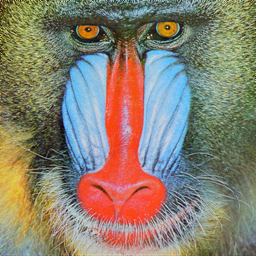
ex2_7プログラム 画像ファイル
カラー信号の色成分分布
% Standard Image? (Mandrill)
clear;
I1=imread('Mandrill.bmp');
figure(1)
imagesc(I1);
I1r=im2double(I1(:,:,1));
I1g=im2double(I1(:,:,2));
I1b=im2double(I1(:,:,3));
I1Y=0.297*I1r+ 0.587*I1g+0.114*I1b;
I1Cb=-0.169*I1r-0.331*I1g+0.5*I1b;
I1Cr=0.5*I1r-0.419*I1g-0.081*I1b;
imwrite(I1Y,'Mandrill_Y.bmp');
imwrite(I1Cb,'Mandrill_Cb.bmp');
imwrite(I1Cr,'Mandrill_Cr.bmp');
figure(2)
imagesc(I1Y);colormap(gray)
figure(3)
imagesc(I1Cb);colormap(gray)
figure(4)
imagesc(I1Cr);colormap(gray)
plot3(I1Cb, I1Cr,I1Y,'.','LineWidth',1)
axis([-0.5 0.5 -0.5 0.5 0 1]);axis square, grid on
xlabel('Cb'); ylabel('Cr');zlabel('Y')
ex2_8プログラム
Cb-Cr空間を用いた肌色領域候補画像の作成
% Standard Image? (Barbara)
clear;
I1=imread('Barbara.bmp');
figure(1)
imagesc(I1);
I1r=im2double(I1(:,:,1));
I1g=im2double(I1(:,:,2));
I1b=im2double(I1(:,:,3));
I1Y=(0.297*I1r+ 0.587*I1g+0.114*I1b)*255;
I1Cb=(-0.169*I1r-0.331*I1g+0.5*I1b)*255+128;
I1Cr=(0.5*I1r-0.419*I1g-0.081*I1b)*255+128;
imwrite(I1Y/255,'Barbara_Y.bmp');
imwrite(I1Cb/255,'Barbara_Cb.bmp');
imwrite(I1Cr/255,'Barbara_Cr.bmp');
% Skin color decision(100<=Cb<=115, 155<=Cr<=170)
for m=1:312
for n=1:261
if((I1Cb(n,m)<100 |I1Cb(n,m)>115) | (I1Cr(n,m)<155 | I1Cr(n,m)>170))
I1Y(n,m)=16;
else
I1Y(n,m)=255;
end
end
end
figure(2)
imagesc(I1Y);colormap(gray)
imwrite(I1Y/255,'Barbara_face.bmp');
% Block Decision(Y_ave in 8x8 block >125)
for m=1:8:305
for n=1:8:254
A=sum(I1Y(n:n+7,m:m+7));
if(sum(A)/64>125)
I1Y(n:n+8,m:m+8)=255;
else
I1Y(n:n+8,m:m+8)=0;
end
end
end
figure(3)
imagesc(I1Y);colormap(gray)
imwrite(I1Y/255,'Barbara_block.bmp');
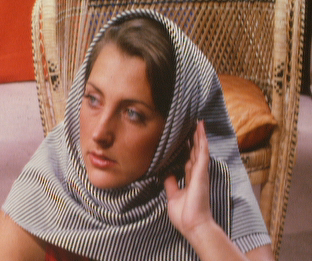
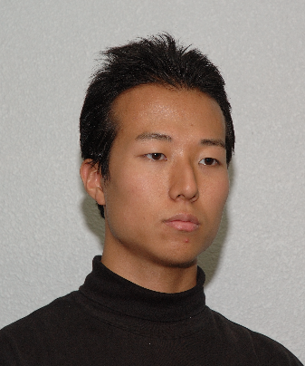
ex2_9プログラム 画像ファイル
ヒストグラムを利用する目と口の領域抽出
% Face Image
clear;
I1=imread('Face.bmp');
figure(1)
imagesc(I1);
I1r=im2double(I1(:,:,1));
I1g=im2double(I1(:,:,2));
I1b=im2double(I1(:,:,3));
I1Y=(0.297*I1r+ 0.587*I1g+0.114*I1b)*255;
I1Cb=(-0.169*I1r-0.331*I1g+0.5*I1b)*255+128;
I1Cr=(0.5*I1r-0.419*I1g-0.081*I1b)*255+128;
imwrite(I1Y/255,'Face_Y.bmp');
imwrite(I1Cb/255,'Face_Cb.bmp');
imwrite(I1Cr/255,'Face_Cr.bmp');
figure(1)
imagesc(I1Y);colormap(gray)
% Luminance Distribution
figure(2)
Y=0:255;
hist(I1Y(:), Y); grid on;
xlabel('Luminance Y');
ylabel('Frequency Distribution D(Y)')
axis([0, 255, 0, 8000])
% Face Area decision(113<=Y<=160)
for m=1:337
for n=1:404
if((I1Y(n,m)<113 |I1Y(n,m)>160))
I1Y(n,m)=16;
else
I1Y(n,m)=255;
end
end
end
figure(3)
imagesc(I1Y);colormap(gray)
imwrite(I1Y/255,'Face_area.bmp');
% Luminance Average along x and y
A=sum(I1Y);
B=sum(I1Y,2);
figure(4)
imagesc(I1Y);colormap(gray)
imwrite(I1Y/255,'barbara256_block.bmp');
x=1:337;
y=1:404;
F=[1 1 1 1 1]/5;
AA=conv(A,F);
D_AA=(diff(AA));
for m=3:339; D_A(m-2)=fix(D_AA(m)); end;
for m=3:335
if((D_A(m)>-1 | D_A(m)<1) & D_A(m-2)<-100 & D_A(m+2)>100 & A(m)>15000)
xp(m)=1;
else
xp(m)=0;
end
end;
xp(1)=0; xp(2)=0; xp(336)=0; xp(337)=0;
BB=conv(B,F);
D_BB=(diff(BB));
for n=3:406; D_B(n-2)=fix(D_BB(n)); end;
for n=3:402
if((D_B(n)>-1 | D_B(n)<1) & D_B(n-2)<-100 & D_B(n+2)>100 & B(n)>15000)
yp(n)=1;
else
yp(n)=0;
end
end;
yp(1)=0; yp(2)=0; yp(403)=0; yp(404)=0;
for n=3:406; D_B(n-2)=D_BB(n); end;
figure(5)
plot(x,A);
grid on;
xlabel('X position');
ylabel('Accumulated Luminance sigma(X)')
axis([1, 337, 0, 50000])
figure(6)
plot(y,B);
grid on;
xlabel('Y position');
ylabel('Accumulated Luminance sigma(Y)')
axis([1, 404, 0, 40000])
figure(7)
subplot(3,2,1);plot(x,A);
subplot(3,2,2);plot(y,B);
subplot(3,2,3);plot(x,D_A);
subplot(3,2,4);plot(y,D_B);
subplot(3,2,5);plot(x,xp);
subplot(3,2,6);plot(y,yp);
%
for m=1:337
if(xp(m)==1)
for n=1:404; I1Y(n,m)=128; end;
end;
end;
for n=1:404
if(yp(n)==1)
for m=1:337; I1Y(n,m)=128; end;
end;
end;
figure(8)
imagesc(I1Y);colormap(gray)
imwrite(I1Y/255,'Face_parts.bmp');
ex2_10プログラム
2次元の特徴量空間における等ユークリッド距離を与える境界
% 2 dimensional Eucledian distance
clear
px=randn(1, 100)-1; py=randn(1,100)-1;
qx=randn(1, 100)+1; qy=randn(1,100)+1;
plot(px,py,'bx');
hold on;
plot(qx,qy, 'gx');
xlabel('feature s1');
ylabel('feature s2');
hold on;
T_px=mean(px); T_py=mean(py);
T_qx=mean(qx); T_qy=mean(qy);
plot(T_px,T_py,'rs');
plot(T_qx,T_qy,'ro');
axis([-5,5,-5,5]);
grid on;
for x=-5:0.1:5
for y=-5:0.1:5
dp=(x-T_px)^2+(y-T_py)^2;
dq=(x-T_qx)^2+(y-T_qy)^2;
if abs(dp-dq)<0.2 plot(x,y,'k.');
end
end
end
hold off;
ex2_11プログラム
2次元の特徴量空間における等マハラノビス距離を与える境界
% 2 dimensional Mahalonobis distance
clear
px=randn(1, 1000)*.8-1; py=randn(1,1000)*0.8-1;
qx=randn(1, 1000)+1; qy=randn(1,1000)+1;
plot(px,py,'bx');
Ap=cov(px,py)
hold on;
plot(qx,qy, 'gx');
Aq=cov(qx,qy)
xlabel('feature s1');
ylabel('feature s2');
hold on;
T_px=mean(px); T_py=mean(py);
T_qx=mean(qx); T_qy=mean(qy);
plot(T_px,T_py,'rs');
plot(T_qx,T_qy,'ro');
axis([-5,5,-5,5]);
grid on;
for x=-5:0.1:5
for y=-5:0.1:5
dp=abs([(x-T_px),(y-T_py)]* inv(Ap) *[(x-T_px),(y-T_py)]');
dq=abs([(x-T_qx),(y-T_qy)]* inv(Aq) *[(x-T_qx),(y-T_qy)]');
if abs(dp-dq)<0.2 plot(x,y,'k.');
end
end
end
hold off;
ex2_12プログラム
50個の2次元特徴量の分布から主軸を求める
% Primary Component Analysis
clear
px=linspace(-2,2,50);
py=linspace(-2,2,50);
px=px+randn(1, 50)*0.2+1; py=py+randn(1,50)*0.5+1;
plot(px,py,'bx');
Ap=cov(px,py);
hold on;
xlabel('feature s1');
ylabel('feature s2');
G_px=mean(px); G_py=mean(py);
plot(G_px,G_py,'ro');
axis([-5,5,-5,5]);
grid on;
ramda1=(Ap(1,1)+Ap(2,2)+sqrt((Ap(1,1)+Ap(1,2))^2-4*(Ap(1,1)*Ap(2,2)-Ap(1,2)^2)))/2;
ramda2=(Ap(1,1)+Ap(2,2)-sqrt((Ap(1,1)+Ap(1,2))^2-4*(Ap(1,1)*Ap(2,2)-Ap(1,2)^2)))/2;
if abs(ramda1)>abs(ramda2)
ramda=ramda1;
else
ramda=ramda2;
end;
a=Ap(1,2)/sqrt(Ap(1,2)^2+(ramda-Ap(1,1))^2);
b=(ramda-Ap(1,2))/sqrt(Ap(1,2)^2+(ramda-Ap(1,1))^2);
for n=1:50
D(n)=a*(px(n)-G_px)+b*(py(n)-G_py);
end;
for x=-5:0.1:5
y=a/b*x;
plot(x,y,'k.');
end
hold off;
ex2_13プログラム
画像の平行移動と回転
% Matching Process
clear
% Test Pattern? (Grating)
clear;
W=128; %横幅
H=256; %縦幅
I1=zeros(H,W);
I_center=128;
I_mod=128;
f_start=40; % 最低空間周波数
f_stop=80; % 最高空間周波数 cycle/W
f_w=f_stop-f_start;
for x=1:W;
for y=1:H;
r=sqrt(((x-64)/W)^2+((y-300)/H)^2);
I1(y,x)=I_center+I_mod*cos((2*pi*f_start+pi*f_w*r^2));
end
end
figure(1)
imagesc(I1,[0,256]);colormap(gray)
imwrite(I1/256,'sim_fing1.bmp');
% 10 pixel moving
I2=zeros(H,W);
for x=1:W;
for y=1:H;
r=sqrt(((x-74)/W)^2+((y-300)/H)^2);
I2(y,x)=I_center+I_mod*cos((2*pi*f_start+pi*f_w*r^2));
end
end
figure(2)
imagesc(I2,[0,256]);colormap(gray)
imwrite(I2/256,'sim_fing2.bmp');
% rotation 10 degree
theta=10;
th=theta/180*pi;
I3=zeros(H,W);
for x=1:W;
for y=1:H;
rx=x*cos(th)+y*sin(th);
ry=-x*sin(th)+y*cos(th);
r=sqrt(((rx-74)/W)^2+((ry-300)/H)^2);
I3(y,x)=I_center+I_mod*cos((2*pi*f_start+pi*f_w*r^2));
end
end
figure(3)
imagesc(I3,[0,256]);colormap(gray)
imwrite(I3/256,'sim_fing3.bmp');
ex2_14プログラム
線形伸縮
% Attenuation signal
alpha=300;????? % alpha:attenuation constant
fc=200;??? % fc:carrier frequency
% obserbvation time: 0 to 20ms
% Number of samples: N1=100samples
N1=100;
t1=linspace(0, 0.02, N1);
s1=exp(-alpha*t1).*sin(2*pi*fc*t1);
figure(1);
plot(t1,s1);grid on
xlabel('Time [sec]');
ylabel('Attenuation signal s1(t)');
% Different frequency : 220Hz
% Different alpha: 330
fc=220;
alpha=330;
N2=100;
t2=linspace(0, 0.02, N2);
s2=exp(-alpha*t2).*sin(2*pi*fc*t2);
figure(2);
plot(t2,s2);grid on
xlabel('Time [sec]');
ylabel('Attenuation signal s2(t)');
% Enlarge 110%
dt2=0.02/(N2-1)*1.1;
t2=t2*1.1;
% Linear interpolation s2(1:100) ==> s3(1:100)
N3=100;
dt1=0.02/(100-1);
for j=1: N3
t3(j)=0.02/(N3)*(j-1);
i=fix(t3(j)/dt2)+1;
a=abs(t2(i)-t3(j))/dt2;
b=abs(t2(i+1)-t3(j))/dt2;
s3(j)=b*s2(i)+a*s2(i+1);
end
figure(3);
plot(t3,s3);grid on
xlabel('Time [sec]');
ylabel('Interporated and Enlarged attenuation signal s3(t)');
ex2_15プログラム
非線形伸縮
% Attenuation signal
alpha=300;????? % alpha:attenuation constant
fc=100;??? % fc:carrier frequency
% obserbvation time: 0 to 20ms
% Number of samples: N1=100samples
N1=100;
t1=linspace(0, 0.02, N1);
s1=exp(-alpha*t1).*sin(2*pi*fc*t1);
figure(1);
plot(t1,s1);grid on
xlabel('Time [sec]');
ylabel('Attenuation signal s1(t)');
% Non-linear time companding signal creation
dt=0.02/(N1-1);
for i=1:100
t2(i)=t1(i)+0.002*sin(2*pi*dt*(i-1)/0.02);
end
s2=exp(-alpha*t2).*sin(2*pi*fc*t2);
figure(2);
plot(t1,s2);grid on
xlabel('Time [sec]');
ylabel('Attenuation signal s2(t)');
figure(3);
plot(t1,t2);grid on
xlabel('t1 [sec]');
ylabel('t2 [sec]');
% DP Matching
err(100,100)=zeros;
err_sum=0;
for i=1:100
for j=1:100
err(i,j)=abs(s1(i)-s2(j));
end
end
s3(1:100)=zeros;
s3(1)=s2(1);
s3(100)=s2(100);
j=2;
for i=2:99
if (err(i,j)<err(i-1,j)) && (err(i,j)<err(i,j-1))
j=i;
elseif (err(i-1,j)<err(i,j)) && (err(i-1,j)<err(i,j-1))
j=i-1;
else
j=j-1;
end
s3(i)=s2(j);
j=j+1;
end
figure(4);
plot(t1,s3);grid on
xlabel('Time [sec]');
ylabel('DP matchedattenuation signal s3(t)');
Copyright コロナ社 All rights reserved.